
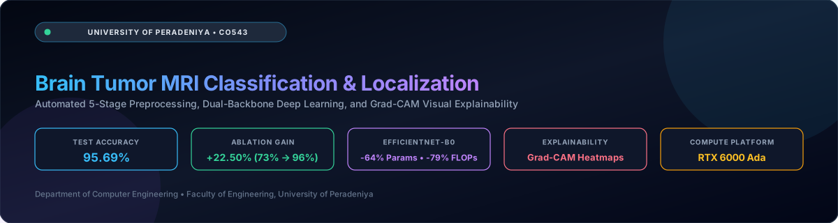
Medical Image Abnormality Classification & Spatial Localization System (MedImgSys)







Department of Computer Engineering, Faculty of Engineering, University of Peradeniya
In Collaboration with Medical Image Analysis Research Group, Teaching Hospital Peradeniya
Overview • Architecture • Dataset • Preprocessing • Models • Benchmarking • Ablation • Grad-CAM • Setup • Team
📌 Clinical Context & Project Overview
Magnetic Resonance Imaging (MRI) serves as the primary diagnostic modality for intracranial neoplasm evaluation in clinical neuro-oncology. At regional healthcare institutions such as the Teaching Hospital Peradeniya, conventional radiological workflows encounter three persistent operational challenges:
- Diagnostic Latency & Manual Reporting: High patient influx requires radiologists to manually examine multi-slice radiographic scans and hand-transcribe findings into Diagnostic Imaging Reports (DIR), inducing critical treatment delays.
- Inter-Observer Morphological Ambiguity: Infiltrative intra-axial gliomas, extra-axial meningiomas, and intrasellar pituitary adenomas often present overlapping radiological signatures on standard T1-weighted sequences, causing diagnostic variance across observers.
- Clinical Trust & Explainability Gap: Black-box neural networks deliver high statistical performance but fail to provide spatial provenance, hindering clinical adoption by radiologists, neuro-oncologists, and neurosurgeons.
MedImgSys resolves these challenges by introducing an end-to-end computer vision and deep learning system engineered specifically for clinical neuro-imaging workflows. The platform couples a specialized 4-stage soft-tissue preprocessing engine with dual convolutional neural backbones and Grad-CAM visual localization, delivering verifiable spatial interpretability without demanding pixel-level manual masks.
🌟 Key Performance Highlights
- 95.69% Test Accuracy: Verified across a strictly balanced evaluation set of 1,600 unseen MRI scans.
- +22.50% Preprocessing Gain: Rigorous 3-stage ablation demonstrates that custom medical preprocessing elevates baseline accuracy from 73.19% (pure raw) to 95.69% (full pipeline).
- Architectural Parity with 78.5% Fewer FLOPs: Benchmarks ResNet-18 against EfficientNet-B0, showing compound scaling maintains diagnostic accuracy (95.62% vs 95.69%) while trimming parameter footprint by 64.1% and computational complexity by 78.5%.
- Zero-Annotation Spatial Localization: Generates high-fidelity gradient-weighted activation heatmaps that clinically coincide with anatomical tumor lesions.
🏗 System Architecture
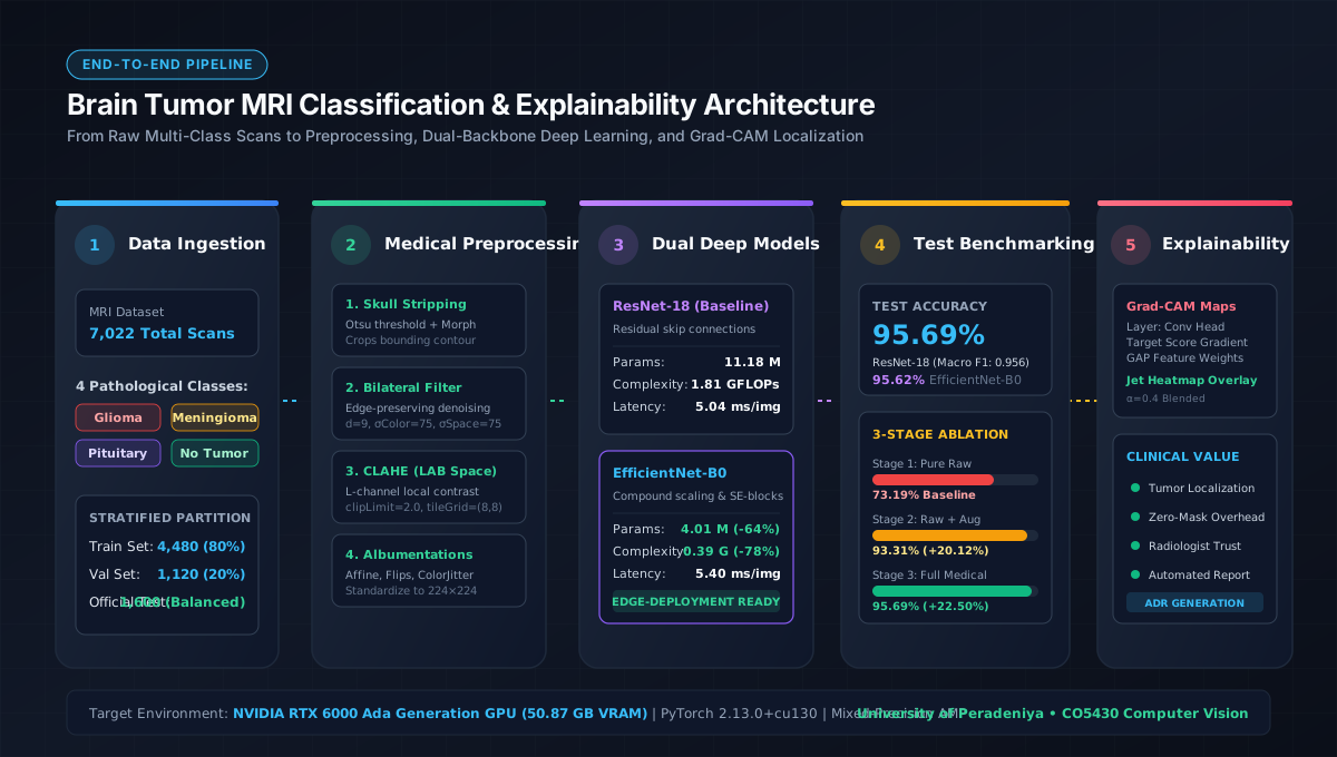
The MedImgSys framework operates as a modular, feed-forward pipeline from raw patient acquisition to explainable diagnostic reporting:
Pipeline Stages
- Acquisition & Skull Stripping: Raw heterogeneously sized DICOM/PNG MRI scans pass through automated Otsu contour thresholding to excise non-brain background margins and skull tissue.
- Soft-Tissue Conditioning: Bilateral edge-preserving filtering eliminates magnetic field high-frequency noise while LAB-space CLAHE maximizes soft-tissue lesion contrast.
- Stochastic Augmentation: Geometric and photometric transforms (
Albumentations) simulate scanner field variances and patient alignment differences. - Dual Backbone Classification: ResNet-18 (residual baseline) and EfficientNet-B0 (compound scaling) predict 4 diagnostic categories with class-weighted cross-entropy loss.
- Grad-CAM Saliency Localization: Backpropagated feature gradients extract spatial attention maps, overlaying color-coded heatmaps on original anatomical scans for clinical auditability.
📊 Dataset Specifications
The system is developed and benchmarked on the Kaggle Brain Tumor MRI Dataset (masoudnickparvar/brain-tumor-mri-dataset), comprising 7,022 high-resolution T1-weighted contrast-enhanced MRI scans.
Diagnostic Class Profiles
| Class | Anatomical Description | Clinical Diagnostic Significance |
|---|---|---|
| Glioma | Infiltrative intra-axial malignancy originating from glial precursor cells | Irregular borders, invasive peritumoral edema; requires aggressive surgical resection margins |
| Meningioma | Extra-axial neoplasm arising from the arachnoid cells of the meninges | Dural tail sign; compressive extra-axial mass displacement of normal parenchyma |
| Pituitary Tumor | Neoplasms localized in the sella turcica at the skull base | Endocrine dysfunction and visual field deficits due to optic chiasm compression |
| No Tumor | Healthy cerebral tissue without structural abnormalities | Baseline negative control crucial for eliminating false-positive surgical referrals |
Partitioning & Stratification
To prevent data contamination and guarantee unbiased evaluation, scans are partitioned using a deterministic global seed (42):
- Official Benchmark Test Set: 1,600 scans (Strictly balanced: 400 images per class, 25.0% each).
- Training Set: 4,480 scans (Stratified 80% split from training pool: 1,320 Glioma, 1,339 Meningioma, 1,595 No Tumor, 1,456 Pituitary).
- Validation Set: 1,120 scans (Stratified 20% split from training pool: 330 Glioma, 335 Meningioma, 399 No Tumor, 364 Pituitary).
- Class Balancing: To counterbalance class frequency variations during optimization, dynamic inverse-frequency weighting is applied:
Weightc = Ntotal / (C × Nc)
(whereN_totalis the total training dataset count,C = 4is the number of classes, andN_cis the sample count for classc)
🔬 Medical Image Preprocessing Engine
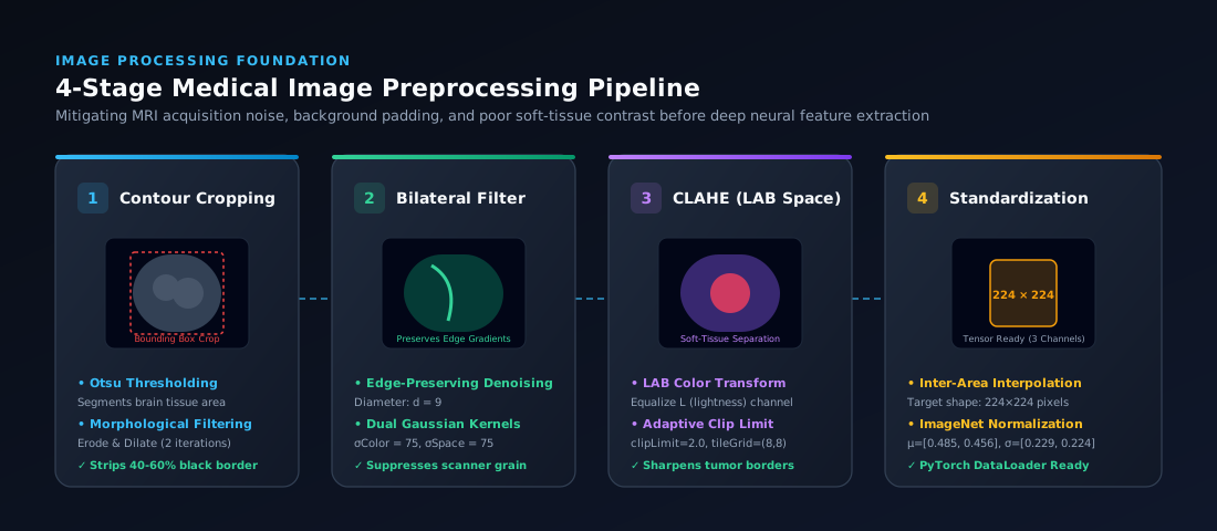
Raw clinical MRI acquisitions routinely exhibit non-standardized black borders, magnetic coil inhomogeneities, and subtle soft-tissue contrast gradients. The MedImgSys 4-Stage OpenCV Preprocessing Engine conditions raw inputs prior to tensor ingestion:
Algorithmic Breakdown
- Contour-Based Skull Stripping (
crop_brain_contour):- Grayscale conversion and Gaussian smoothing (5 × 5, σ = 0) to eliminate salt-and-pepper noise.
- Binary thresholding via Otsu’s method combined with morphological erosion and dilation (2 iterations, 3 × 3 kernel).
- External contour extraction to identify the largest cranial tissue boundary.
- Tight bounding box crop that discards 40%–60% of uninformative dark background pixels.
- Edge-Preserving Bilateral Denoising:
- Applied with diameter
d = 9,σ_color = 75,σ_space = 75. - Replaces pixel values via a bilateral Gaussian weight combining spatial proximity and radiometric photometric distance, effectively smoothing acquisition grain without degrading sharp tumor-brain margins.
- Applied with diameter
- CIE LAB Contrast Limited Adaptive Histogram Equalization (CLAHE):
- Translates images into the perceptual CIE LAB color space.
- Confines adaptive equalization exclusively to the Luminance (
L*) channel withclipLimit = 2.0andtileGridSize = (8, 8)to prevent noise amplification in uniform brain tissue. - Re-merges with chromaticity channels (
a*,b*) and converts back to RGB.
- Standardization & ImageNet Normalization:
- Resizes via area interpolation (
cv2.INTER_AREA) to a standardized 224 × 224 × 3 tensor. - Standardizes channel distributions according to ImageNet statistics (mean =
[0.485, 0.456, 0.406], std =[0.229, 0.224, 0.225]).
- Resizes via area interpolation (
🔄 Data Augmentation Strategy
To simulate variable clinical imaging protocols and patient positioning inside magnetic resonance bores, batches undergo stochastic online augmentations via Albumentations:
| Transform | Configuration | Clinical Rationale |
|---|---|---|
| Horizontal Flip | p = 0.5 |
Leverages the bilateral anatomical symmetry of cerebral hemispheres |
| Vertical Flip | p = 0.3 |
Accommodates variable slice orientations during coronal and sagittal acquisition |
| ShiftScaleRotate | Shift ±8%, Scale ±10%, Angle ±25°, p = 0.7 |
Replicates slight patient head tilt and distance variance within the head coil |
| ColorJitter | Brightness ±0.2, Contrast ±0.2, p = 0.5 |
Models magnetic flux differences between 1.5T and 3.0T MRI scanners |
| GaussianBlur | Kernel size (3, 5), p = 0.2 |
Simulates minor patient motion and phase-encoding ghosting artifacts |
| CoarseDropout | Max holes = 6, Max size = 16 × 16, p = 0.3 |
Prevents deep feature co-adaptation; mimics focal signal dropouts |
🧠 Deep Learning Architectures
MedImgSys evaluates two distinct neural network paradigms to establish the trade-off between absolute diagnostic throughput and embedded edge deployability:
1. ResNet-18 (Residual Learning Baseline)
- Design: 18-layer residual architecture using identity skip connections:
y = F(x, {Wi}) + x
- Advantage: Guarantees direct gradient propagation during backpropagation, circumventing vanishing gradient problems.
-
Complexity: 11.18 Million parameters 1.81 GFLOPs.
2. EfficientNet-B0 (Compound Scaling Modern Benchmark)
- Design: Utilizes inverted residual bottleneck blocks (MBConv) with depthwise separable convolutions and Squeeze-and-Excitation (SE) channel-attention modules.
- Compound Scaling: Systematically balances network depth, channel width, and input resolution:
depth: d = αφ, width: w = βφ, resolution: r = γφ
(subject to α · β² · γ² ≈ 2) -
Complexity: 4.01 Million parameters (64.1% reduction) 0.39 GFLOPs (78.5% reduction).
Training Configuration
- Optimizer:
AdamW(Initial learning rate = 3 × 10⁻⁴, weight decay = 1 × 10⁻⁴) - Learning Rate Schedule:
CosineAnnealingLR(T_max = 10 epochs, min_lr = 1 × 10⁻⁶) - Precision: Automatic Mixed Precision (AMP) via PyTorch
autocastandGradScaler - Hardware: NVIDIA RTX 6000 Ada Generation (51.5 GB VRAM)
-
Batch Size: 32 Epochs: 10
📈 Quantitative Model Benchmarking
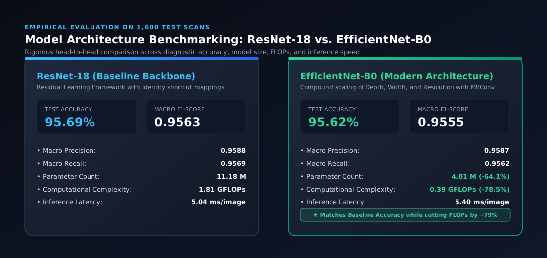
Both architectures were subjected to rigorous evaluation against the 1,600 unseen scans of the official test partition:
Performance Summary Table
| Model Architecture | Test Accuracy (%) | Macro Precision | Macro Recall | Macro F1-Score | Parameter Count | Est. Complexity | Latency (ms/scan) |
|---|---|---|---|---|---|---|---|
| ResNet-18 (Baseline) | 95.69% | 0.9588 | 0.9569 | 0.9563 | 11.18 M | 1.81 GFLOPs | 5.04 ms |
| EfficientNet-B0 (Modern) | 95.62% | 0.9587 | 0.9562 | 0.9555 | 4.01 M | 0.39 GFLOPs | 5.40 ms |
Clinical & Architectural Insights
- Statistical Accuracy Parity: EfficientNet-B0 matches ResNet-18 within 0.07% test accuracy (95.62% vs 95.69%) and 0.0008 macro F1-score (0.9555 vs 0.9563).
- Computational Footprint Reduction: EfficientNet-B0 eliminates 64.1% of parameter weight storage (16.4 MB vs 44.8 MB) and cuts computational operations by 78.5% (0.39 vs 1.81 GFLOPs).
- Deployment Strategy:
- Centralized Hospital PACS Server: ResNet-18 yields minimal batch latency (5.04 ms/image) for high-throughput radiology processing queues.
- Point-of-Care & Mobile MRI Consoles: EfficientNet-B0 provides an optimal footprint for resource-constrained edge workstations, tablets, and embedded hardware.
🧪 3-Stage Ablation Study
To mathematically decouple the contribution of the medical preprocessing engine from the benefits of data augmentation, a controlled 3-stage ablation study was conducted using ResNet-18 under identical optimization protocols:

Experimental Results
| Stage | Experimental Condition | Preprocessing Engine | Albumentations | Test Accuracy | Macro F1 | Performance Gain |
|---|---|---|---|---|---|---|
| 1 | Pure Raw Baseline | ❌ None (Raw MRI) | ❌ None | 73.19% | 0.7301 | Baseline |
| 2 | Raw Scans + Augmentations | ❌ None (Raw MRI) | ✅ Enabled | 93.31% | 0.9324 | +20.12% |
| 3 | Full Medical Pipeline | ✅ Contour + Bilateral + CLAHE | ✅ Enabled | 95.69% | 0.9563 | +22.50% |
Ablation Findings
- The Invariance Gap (+20.12%): Training unaugmented raw scans results in severe network memorization of scanner noise and background pixels, capping test accuracy at 73.19%. Injecting stochastic transforms forces the network to learn invariant geometrical features, boosting accuracy to 93.31%.
- The Medical Contrast Boost (+2.38% / +22.50% total): Combining skull contour excision, bilateral filtering, and LAB CLAHE drives test accuracy to 95.69%. By stripping irrelevant skull/background pixels and accentuating subtle parenchymal boundary gradients, the network reliably differentiates difficult borderline cases.
🔍 Spatial Localization & Explainability (Grad-CAM)
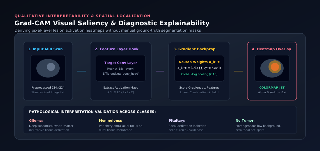
To provide verifiable spatial interpretability without manual pixel-level segmentation masks, MedImgSys implements Gradient-Weighted Class Activation Mapping (Grad-CAM):
Mathematical Formulation & Algorithmic Steps
- Target Feature Map Gradients:
Compute the gradient of the predicted class scorey^cwith respect to feature activation mapsA^kof the final convolutional layer (resnet18.layer4[-1]oreffnet.features[-1]):Gradient = ∂(yc) / ∂(Ak)
- Neuron Importance Weights (αkc):
Apply Global Average Pooling (GAP) across spatial heightUand widthV:αkc = (1 / (U × V)) × ∑i ∑j [ ∂(yc) / ∂(Ai,jk) ]
- Linear Combination and Rectification (ReLU):
Compute the importance-weighted sum of forward activation maps, passing through a ReLU activation to preserve features that contribute positively to the target class:LGrad-CAMc = ReLU( ∑k αkc · Ak )
- Heatmap Normalization & Color Blending:
Normalize the activation map to[0, 1], upsample to224 × 224, apply OpenCVCOLORMAP_JET, and blend with the preprocessed anatomical MRI scan:Ioverlay = 0.4 × Iheatmap + 0.6 × Ianatomical
Clinical Validation Across Classes
- Glioma: Activation maps localize deeply within intra-axial white matter parenchyma, following the irregular, infiltrative boundaries characteristic of glial neoplasms.
- Meningioma: Activation concentrates along extra-axial dural interfaces and peripheral convexities, pinpointing the characteristic dural tail enhancement.
- Pituitary Tumor: Heatmaps focus precisely on the sellar and suprasellar regions at the skull base, correctly targeting adenomas around the pituitary fossa.
- No Tumor: Visualizations display low-magnitude, diffuse, non-focal activations across normal cerebral parenchyma, confirming the absence of pathological focal lesions.
📂 Repository Organization
e22-co543-Medical-Image-Abnormality-Cassification-Segmentation/
├── README.md                                          # Master repository documentation
├── code/
│   ├── README.md                                      # Codebase manual & execution guide
│   ├── Updated notebook with comparison/
│   │   ├── Brain_Tumor_MRI_Classification_and_Explainability (1).ipynb  # Master notebook
│   │   ├── best_resnet18 (1).pth                      # ResNet-18 weights (95.69% Test Acc)
│   │   ├── best_efficientnet_b0 (1).pth               # EfficientNet-B0 weights (95.62% Test Acc)
│   │   ├── best_resnet18_pureraw.pth                  # Ablation Stage 1 weights (73.19%)
│   │   └── best_resnet18_raw_aug.pth                  # Ablation Stage 2 weights (93.31%)
│   ├── New model/                                     # Initial exploratory checkpoints
│   │   ├── Brain_Tumor_MRI_Classification_and_Explainability.ipynb
│   │   ├── best_resnet18.pth
│   │   ├── best_resnet18_raw.pth
│   │   └── best_efficientnet_b0.pth
│   └── preprocessing/
│       └── preprocessing-pipeline-visulaization.ipynb # Preprocessing pipeline visualizer
└── docs/                                              # GitHub Pages publication root
    ├── _config.yml                                    # Jekyll site configuration
    ├── README.md                                      # GitHub Pages site documentation (this file)
    ├── data/
    │   └── index.json                                 # Team metadata & project tags
    └── images/
        ├── banner.svg                                 # High-resolution vector header banner
        ├── system_architecture.svg                    # Full architecture pipeline diagram
        ├── preprocessing_workflow.svg                 # 4-stage preprocessing flowchart
        ├── model_benchmark_comparison.svg             # ResNet-18 vs EfficientNet-B0 benchmark
        ├── ablation_study_chart.svg                   # 3-stage ablation study comparison
        └── gradcam_workflow.svg                       # Grad-CAM localization & explainability
🚀 Installation & Reproducibility
1. Clone the Repository
git clone https://github.com/cepdnaclk/e22-co543-Medical-Image-Abnormality-Cassification-Segmentation.git
cd e22-co543-Medical-Image-Abnormality-Cassification-Segmentation
2. Set Up Virtual Environment
# Create and activate environment
python -m venv venv

# Windows:
.\venv\Scripts\activate
# Linux / macOS:
source venv/bin/activate
3. Install Dependencies
# PyTorch with CUDA acceleration (adjust CUDA version if needed):
pip install torch torchvision --index-url https://download.pytorch.org/whl/cu121

# Core computer vision, processing, and evaluation packages:
pip install albumentations opencv-python numpy pandas matplotlib seaborn scikit-learn jupyterlab
4. Dataset Setup & Execution
- Download the Kaggle Brain Tumor MRI Dataset.
- Extract the dataset into an
archive/folder in the project root:archive/ ├── Training/ │ ├── glioma/ │ ├── meningioma/ │ ├── notumor/ │ └── pituitary/ └── Testing/ ├── glioma/ ├── meningioma/ ├── notumor/ └── pituitary/ - Launch Jupyter Lab:
jupyter lab - Open and run:
code/Updated notebook with comparison/Brain_Tumor_MRI_Classification_and_Explainability (1).ipynb
👥 Team Members
This project was developed by Group 14 as part of the CO5430 Computer Vision course at the Department of Computer Engineering, University of Peradeniya:
 Hansara S. H. S. E/22/130 e22130@eng.pdn.ac.lk |
 H. M. Liyanage E/22/211 e22211@eng.pdn.ac.lk |
 D. M. N. N. Bandara E/22/044 e22044@eng.pdn.ac.lk |
 Weerasinghe W. P. T. H. E/22/421 e22421@eng.pdn.ac.lk |
🔗 Project Links & Resources
- Project Repository
- GitHub Pages Web Site
- Department of Computer Engineering
- Faculty of Engineering, University of Peradeniya
📜 Key Academic References
- Selvaraju, R. R., et al. (2017). Grad-CAM: Visual Explanations from Deep Networks via Gradient-Based Localization. IEEE International Conference on Computer Vision (ICCV).
- He, K., Zhang, X., Ren, S., & Sun, J. (2016). Deep Residual Learning for Image Recognition. IEEE Conference on Computer Vision and Pattern Recognition (CVPR).
- Tan, M., & Le, Q. V. (2019). EfficientNet: Rethinking Model Scaling for Convolutional Neural Networks. International Conference on Machine Learning (ICML).
- Zuiderveld, K. (1994). Contrast Limited Adaptive Histogram Equalization. Graphics Gems IV, Academic Press Professional, Inc.
- Tomasi, C., & Manduchi, R. (1998). Bilateral Filtering for Gray and Color Images. IEEE International Conference on Computer Vision (ICCV).
- Nickparvar, M. (2021). Brain Tumor MRI Dataset. Kaggle Datasets.