Click the thumbnail above to watch the video lecture on YouTube
12.1 Introduction
This lecture introduces pipelining as the primary performance enhancement technique in modern processor design, transforming the inefficient single-cycle architecture into a high-throughput execution engine. We explore how pipelining applies assembly-line principles to instruction execution, dramatically improving processor throughput while maintaining individual instruction latency. The lecture examines the three fundamental types of hazards—structural, data, and control—that threaten pipeline efficiency, and discusses practical solutions including forwarding, stalling, and branch prediction that enable real-world pipelined processors to achieve near-ideal performance.
12.2 Recap: Single-Cycle Performance Limitations
12.2.1 Critical Path Problem
Load Word as Bottleneck:
- Uses most resources: Instruction Memory → Register File → ALU → Data Memory → Register File
- Determines clock period for entire CPU
- Forces all other instructions to wait
Performance Issue:
- Most instructions (arithmetic, branch) take less time than load
- Jump instruction takes even less time
- Clock period set by slowest instruction (load word)
Design Principle Violated:
- "Make the common case fast"
- Common case (arithmetic) forced to run slowly
- Majority of instructions underutilize available time
12.2.2 Multi-Cycle as First Improvement
Basic Concept:
- Divide datapath into stages
- Each stage completes in one clock cycle
- Shorter clock cycles than single-cycle
Five Stages Identified:
- Instruction Fetch (IF)
- Register Reading
- ALU Operations
- Memory Access
- Register Writing
Variable Stage Usage:
- Load: Uses all 5 stages
- Most instructions: Skip memory access (4 stages)
- Jump: Only 2 stages (manipulating PC)
Clock Period Determination:
- Decided by slowest stage (not slowest instruction)
- Adjust work in each stage for balance
- Maximize utilization of each clock cycle
Limitation:
- Instruction must finish before next instruction starts
- Hardware still idle during many cycles
- Room for further improvement
12.3 Pipelining Concept: The Laundry Shop Analogy
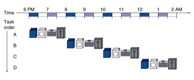
12.3.1 Non-Pipelined Laundry Shop
Setup:
- One employee
- Four customers: A, B, C, D
- First-come, first-serve basis
- Four stages of work per customer:
- Washing: 30 minutes
- Drying: 30 minutes
- Folding/Ironing: 30 minutes
- Packaging: 30 minutes
- Total per customer: 2 hours
Sequential Processing:
| Metric | Value |
|---|---|
| Total Time | 8 hours (6pm to 2am) |
| Time per Customer | 2 hours |
| Shop Closes | 2am |
Problems:
- Machines idle while employee works on other stages
- Washer idle during drying, folding, packaging
- Dryer idle except during drying stage
- Tremendous resource underutilization
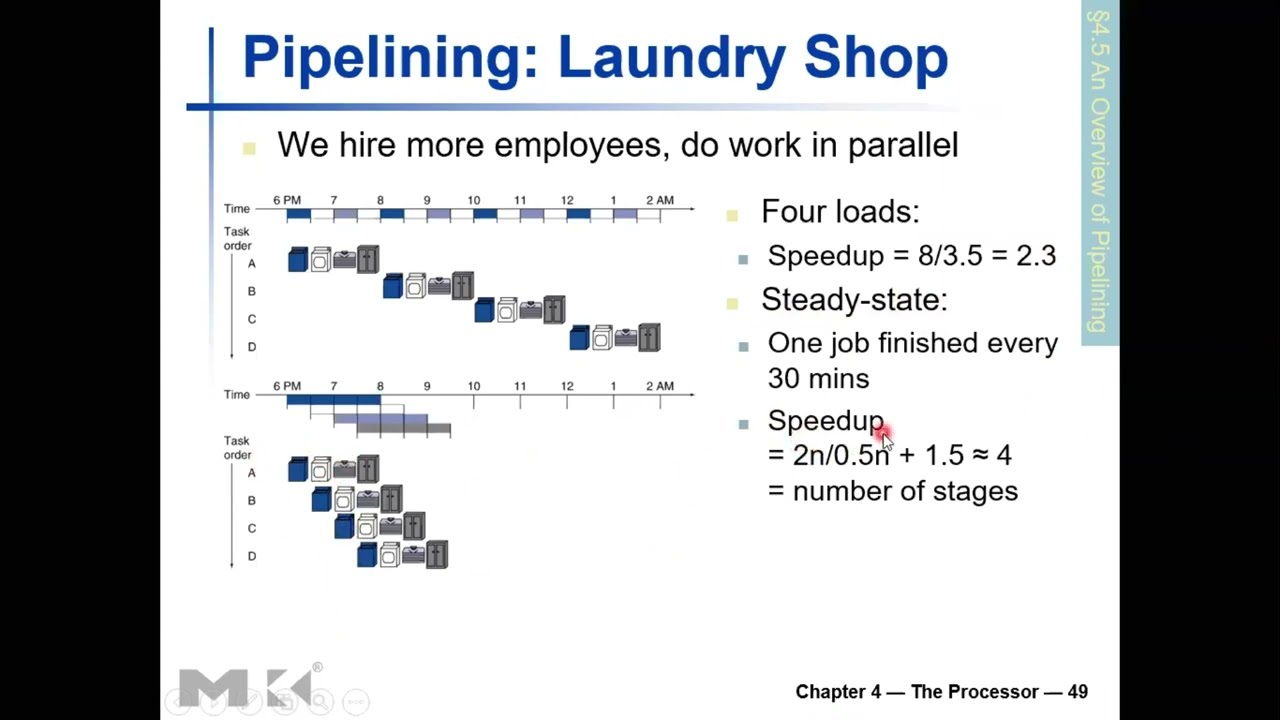
12.3.2 Pipelined Laundry Shop
Key Idea:
- Use idle machines for next customers
- Overlap execution of different loads
- Parallel processing maximizes hardware utilization
Pipelined Schedule:
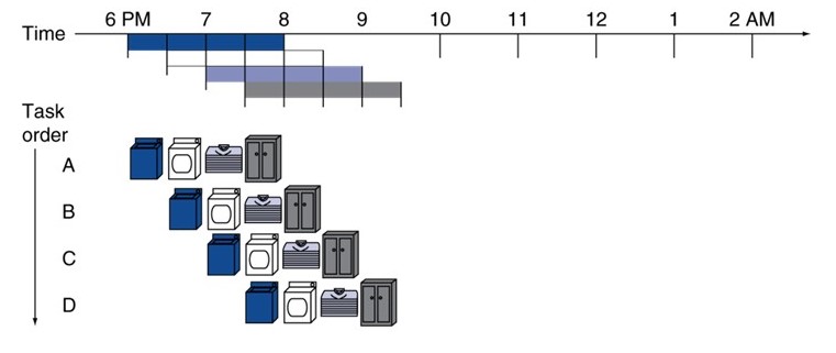
Timeline Analysis:
- 6:00-6:30: A washing (1 station busy)
- 6:30-7:00: A drying, B washing (2 stations busy)
- 7:00-7:30: A folding, B drying, C washing (3 stations busy)
- 7:30-8:00: A packing, B folding, C drying, D washing (4 stations - ALL BUSY!)
- 8:00-8:30: A done, B packing, C folding, D drying, E washing
Steady State:
- Reached at 7:30-8:00 when all 4 stations occupied
- Pipeline full
- Maximum hardware utilization
- One customer finishes every 30 minutes
12.3.3 Performance Analysis
Time Comparison:
- Non-pipelined: 8 hours for 4 customers
- Pipelined: 3.5 hours for 4 customers
Speedup Calculation:
Speedup = Non-pipelined Time / Pipelined Time
        = 8 hours / 3.5 hours
        = 2.3×
Includes Pipeline Fill Time:
- First 1.5 hours: Filling pipeline (not all stations busy)
- After 1.5 hours: Steady state (all stations busy)
Steady State Analysis (ignoring fill time):
Non-pipelined: 2n hours for n loads (2 hours per load)
Pipelined: 0.5n hours for n loads (0.5 hours per load)

Steady State Speedup = 2n / 0.5n = 4×
Theoretical Maximum Speedup:
- Equals number of stages
- 4 stages → 4× speedup maximum
- 8 stages → 8× speedup maximum (if achievable)
12.3.4 Key Performance Terms
Latency:
- Time to complete one individual job
- Customer A: Still 2 hours in both cases
- Per-instruction time unchanged
Throughput:
- How often one job completes
- Non-pipelined: 1 job every 2 hours
- Pipelined: 1 job every 30 minutes (steady state)
- Throughput is the relevant metric for pipelines
Observation:
- Pipelining doesn't reduce individual job latency
- Pipelining dramatically improves throughput
- Overall system performance greatly enhanced
Analogy Summary:
- Customers = Instructions
- Stages = Pipeline stages
- Time saved = Performance improvement
- Overlapping execution = Instruction-level parallelism
12.4 MIPS Five-Stage Pipeline
12.4.1 Pipeline Stage Definitions
Stage 1: Instruction Fetch (IF)
- Use current Program Counter (PC)
- PC points to next instruction to execute
- Access instruction memory
- Fetch instruction word
- Duration: One clock cycle
Stage 2: Instruction Decode / Register Read (ID)
- Decode opcode field
- Determine instruction category
- Identify remaining bit organization
- Extract register addresses
- Read register file
- Both operations in one stage (workload balancing)
Stage 3: Execution (EX)
- Arithmetic/Logic instructions: ALU computes result
- Memory instructions: ALU computes address (base + offset)
- Branch instructions: ALU performs comparison
- One clock cycle
Stage 4: Memory Access (MEM)
- Load instructions: Read from data memory
- Store instructions: Write to data memory
- Other instructions: Skip this stage
- One clock cycle
Stage 5: Write Back (WB)
- Write result to register file
- Source: ALU result (arithmetic) OR memory data (load)
- Multiplexer selects appropriate source
- One clock cycle
Workload Distribution Goal:
- Evenly distribute work across stages
- Minimize clock cycle time
- Maximize hardware utilization
12.4.2 Stage Timing Example
Assumed Component Delays:
| Component | Delay (picoseconds) |
|---|---|
| Instruction Fetch | 200 ps |
| Register Read/Write | 100 ps |
| ALU Operation | 200 ps |
| Data Memory Access | 200 ps |
| Sign Extension | negligible |
| Multiplexers | negligible |
Single-Cycle Instruction Times:
| Instruction Type | Stages Used | Total Time |
|---|---|---|
| Load Word (LW) | IF+ID+EX+MEM+WB | 800 ps |
| Store Word (SW) | IF+ID+EX+MEM | 700 ps |
| R-type (ADD, etc.) | IF+ID+EX+WB | 600 ps |
| Branch (BEQ) | IF+ID+EX | 500 ps |
12.4.3 Pipeline Implementation Details
Clock Cycle Determination:
- Must accommodate longest stage
- Longest stage: 200 ps (IF, ALU, MEM)
- Clock cycle: 200 ps
- Some stages underutilize cycle (register read/write: 100 ps)
Register Read/Write Timing:
- CRITICAL: Register write first half, read second half of same clock cycle
- Enables same-cycle read-after-write
- Prevents data hazards in some cases
Stage Alignment to Clock Cycles:
| Stage | Work | Time | Cycle Time |
|---|---|---|---|
| IF | Instruction Memory read | 200 ps | 200 ps ✓ |
| ID | Decode + Register Read | 100 ps | 200 ps (space left) |
| EX | ALU operation | 200 ps | 200 ps ✓ |
| MEM | Data Memory access | 200 ps | 200 ps ✓ |
| WB | Register write | 100 ps | 200 ps (first half only) |
Space in ID Stage:
- Register read: 100 ps
- Decoding: Fits in remaining 100 ps
- Combinational logic for opcode decode
- Total: ~200 ps utilized
Space in WB Stage:
- Register write: 100 ps (first half)
- Second half: Available for next instruction's register read
12.4.4 Load Word Pipeline Example
Instruction Stream: All Load Word instructions
LW $1, 0($10)
LW $2, 4($10)
LW $3, 8($10)
LW $4, 12($10)
...
Pipeline Timing Diagram:
Time (ps):  0-200  200-400  400-600  600-800  800-1000  1000-1200
LW $1:      IF     ID       EX       MEM      WB
LW $2:             IF       ID       EX       MEM       WB
LW $3:                      IF       ID       EX        MEM
LW $4:                               IF       ID        EX
Single-Cycle Comparison:
- Non-pipelined: 800 ps per instruction
- Pipelined: 200 ps per instruction (after pipeline fills)
Throughput Improvement:
Non-pipelined: 1 instruction every 800 ps
Pipelined: 1 instruction every 200 ps

Speedup = 800 / 200 = 4×
Absolute Time per Instruction:
- Still ~800 ps (slightly more with alignment overhead)
- Latency unchanged or slightly worse
- Throughput dramatically improved
12.4.5 Ideal vs Actual Speedup
Ideal Case (balanced stages):
Time between instructions (pipelined) = Time per instruction (non-pipelined) / Number of stages

Maximum Speedup = Number of Stages
Actual Implementation:
- Stages not perfectly balanced
- Register operations faster than memory/ALU
- Speedup < Number of stages
- Example: 5 stages → 4× speedup (not 5×)
Reasons for Less Than Ideal:
- Unbalanced stage delays
- Pipeline fill time overhead
- Hazards (discussed later)
- Added synchronization logic
12.5 MIPS ISA Design for Pipelining
12.5.1 Fixed Instruction Length
MIPS Characteristic:
- All instructions exactly 32 bits
- Same as ARM (also designed for pipelining)
Benefits for Pipelining:
- Simple instruction fetch (always 32 bits)
- Simple decode (fixed format)
- Bus width fully utilized every time
- No variable-width handling logic
Alternative (Variable-Length):
- Complicates fetch stage
- Requires width detection logic
- May need multiple fetch cycles
- Added combinational logic delays
12.5.2 Fewer Regular Instruction Formats
MIPS Formats:
- Only 3-4 instruction formats (R, I, J types)
- Small opcode field (6 bits)
- Regular register field positions
Benefits:
- Fast decoding (small opcode → simple logic)
- Fits decode + register read in one stage
- Minimal combinational delay
Register Field Consistency:
- RS (bits 21-25): First source register
- RT (bits 16-20): Second source / destination
- RD (bits 11-15): Destination (R-type)
- Same positions across formats
Decoding Simplification:
- Small opcode → simple decode logic
- Regular formats → minimal mux complexity
- Fast enough for single clock cycle
12.5.3 Separate ALU Operation Field
Function Field (funct):
- Bits 0-5: Specifies ALU operation for R-type
- Separate from opcode
- Only examined for R-type (opcode = 0)
Design Rationale:
- ALU operation determined in EX stage
- Opcode used in ID stage
- Temporal separation matches pipeline stages
Benefit:
- funct field processed later (EX stage)
- Opcode processed early (ID stage)
- Separating them simplifies each stage
- Avoids large opcode (keeps decode simple)
Alternative Design:
- Include funct in opcode
- Larger opcode field needed
- More complex decode logic
- Slower ID stage
- Worse pipeline balance
12.5.4 Load/Store Addressing Mode
MIPS Addressing:
- Base register + offset
- Address = $rs + immediate
- Calculation: Simple addition
Pipeline Fit:
- Address calculation: EX stage (ALU)
- Memory access: MEM stage (next cycle)
- Clean separation into two stages
Design Philosophy:
- ISA designed with pipeline in mind
- Not optimized for single-cycle
- Performance through pipelining
MIPS vs Other ISAs:
- MIPS: Designed for pipelining from start
- x86: Complex instructions, harder to pipeline
- ARM: Similar philosophy to MIPS
- RISC principles support pipelining
12.6 Instruction-Level Parallelism (ILP)
12.6.1 Parallel Execution Concept
Definition:
- Multiple instructions executing simultaneously
- Each at different pipeline stage
- Overlapping execution
Example at Steady State:
Time Window: 800-1000 ps

Instruction A: WB stage (writing result)
Instruction B: MEM stage (memory access)
Instruction C: EX stage (ALU operation)
Instruction D: ID stage (decode, register read)
Instruction E: IF stage (fetch)

Five instructions active simultaneously!
Instruction-Level Parallelism (ILP):
- Lowest granularity of parallelism
- Inside CPU microarchitecture
- Transparent to software
- Hardware manages parallelism
12.6.2 Levels of Parallelism
Instruction-Level Parallelism:
- Multiple instructions in pipeline
- Same program/thread
- Within CPU core
- Microsecond/nanosecond scale
Thread-Level Parallelism:
- Multiple threads on same core
- Context switching
- OS-managed
- Millisecond scale
Program-Level Parallelism:
- Multiple programs/processes
- Multi-core execution
- OS-scheduled
- Varied time scales
Application-Level Parallelism:
- Distributed computing
- Multiple machines
- Network communication
- Seconds to minutes scale
ILP Focus:
- Fine-grained parallelism
- Hardware implementation
- Transparent to programmer (mostly)
- Foundation for all higher levels
12.7 Pipeline Hazards: Structural Hazards
12.7.1 Hazard Definition
General Concept:
- Situations preventing next instruction from starting
- Violates basic pipelining goal
- Reduces throughput
- Requires pipeline stalls (bubbles)
Three Categories:
- Structural Hazards: Hardware resource busy
- Data Hazards: Need data from previous instruction
- Control Hazards: Decision depends on previous result
12.7.2 Structural Hazard: Single Memory
Scenario:
- Single memory device for both instructions and data
- No separate instruction/data memory
- Same device holds program and data
Conflict Example:
Time:    0-200   200-400  400-600  600-800
LW $1:   IF      ID       EX       MEM
LW $2:           IF       ID       EX
LW $3:                    IF       ID
LW $4:                             IF  ← CONFLICT!

At 600-800 ps:
• LW $1 needs data memory (MEM stage)
• LW $4 needs instruction memory (IF stage)
• Same physical memory device!
• Cannot access simultaneously
Problem:
- Memory can only service one request per cycle
- Instruction fetch AND data access conflict
- Hardware resource (memory) busy
12.7.3 Pipeline Stall (Bubble)
Solution: Insert Bubble
Time:    0-200   200-400  400-600  600-800  800-1000  1000-1200
LW $1:   IF      ID       EX       MEM      WB
LW $2:           IF       ID       EX       [BUBBLE]  MEM
LW $3:                    IF       ID       EX        [BUBBLE]
LW $4:                             IF       [BUBBLE]  ID
Bubble Characteristics:
- No instruction in that pipeline stage
- Like air bubble in water pipeline
- Hardware idle for that stage
- Wastes one clock cycle
- Propagates through pipeline stages
Impact:
- One instruction delayed
- Subsequent instructions delayed
- Throughput reduced
- Performance loss
Bubble Analogy:
- Water pipeline: Continuous flow
- Air bubble: Break in flow
- Takes time to propagate through
- Reduces effective flow rate
12.7.4 Solutions to Structural Hazards
Solution 1: Separate Memories
- Instruction memory separate from data memory
- Harvard architecture
- Simultaneous access possible
- No structural hazard
Solution 2: Separate Caches
- Single main memory
- Separate instruction cache (I-cache)
- Separate data cache (D-cache)
- Cache: Fast buffer between CPU and memory
- Caches can be accessed simultaneously
- Details in future lectures (memory hierarchy)
Design Recommendation:
- Modern processors use separate caches
- Necessary for high-performance pipelining
- Small area overhead for large performance gain
12.8 Data Hazards
12.8.1 Data Hazard Definition
Concept:
- Subsequent instruction needs data from previous instruction
- Data not yet available (still being computed/written)
- Reading too early → wrong value
- Writing too early → data corruption
Example:
ADD $s0, $t0, $t1      # $s0 = $t0 + $t1
SUB $t2, $s0, $t3      # $t2 = $s0 - $t3 (uses $s0 from ADD)
Problem:
- ADD computes $s0 value in EX stage
- SUB needs $s0 value in ID stage (register read)
- Timing mismatch
12.8.2 Data Hazard Example Analysis
Instruction Sequence:
ADD $s0, $t0, $t1
SUB $t2, $s0, $t3
Pipeline Without Stalls:
Time:    0-200   200-400  400-600  600-800  800-1000
ADD:     IF      ID       EX       MEM      WB
SUB:             IF       ID       EX       MEM
                          ↑
                 Reads $s0 here (old value!)

                          ADD writes $s0 here ↓
Problem Timeline:
- 200-400: ADD reads $t0, $t1; SUB fetched
- 400-600: ADD computes in ALU; SUB reads registers (gets OLD $s0!)
- 600-800: ADD result available but not in register yet
- 800-1000: ADD writes $s0 to register (first half of cycle)
SUB reads $s0 at 400-600, but correct value not available until 800-1000!
12.8.3 Solution 1: Pipeline Stalls
Insert Two Bubbles:
Time:    0-200   200-400  400-600  600-800  800-1000  1000-1200  1200-1400
ADD:     IF      ID       EX       MEM      WB
[BUBBLE]                  IF       [BUBBLE] [BUBBLE]
[BUBBLE]                           IF       [BUBBLE]
SUB:                                         IF        ID
Result:
- SUB fetched at 1000-1200
- SUB reads registers at 1200-1400 (second half at 1200)
- ADD writes $s0 at 800-1000 (first half at 800)
- Sufficient time gap: Correct value available
Cost:
- Two clock cycles wasted
- Throughput reduced
- Performance penalty
Critical Timing:
- Register write: First half of WB cycle
- Register read: Second half of ID cycle
- Enables back-to-back reading of just-written value
12.8.4 Solution 2: Forwarding (Bypassing)
Key Observation:
- ADD result available after EX stage (400-600)
- Result at ALU output
- Not yet written to register file
- But SUB's ALU operation at 600-800
- Can forward ALU output directly to ALU input!
Forwarding Logic:
Time:    0-200   200-400  400-600  600-800  800-1000
ADD:     IF      ID       EX       MEM      WB
SUB:             IF       ID       EX       MEM
                          ↑        ↑
                 Read regs   Use forwarded value!
Implementation:
- Multiplexer at ALU input
- Selects between:
- Register file output (normal path)
- Forwarded value from previous ALU output
- Control logic detects dependency
- Routes correct value
Benefit:
- Eliminates two stalls
- No performance penalty
- Requires additional hardware:
- Forwarding multiplexers
- Forwarding detection logic
- Forwarding paths (wires)
- Pipeline registers to hold values
Complexity:
- Careful synchronization required
- Detect true dependencies
- Avoid false positives
- Additional control signals
Result:
- SUB can execute immediately after ADD
- No stalls needed
- Correct value forwarded
12.8.5 Load-Use Data Hazard
Special Case:
LW  $s0, 0($t0)        # Load from memory into $s0
SUB $t2, $s0, $t3      # Use $s0 immediately
Problem:
- Load result available after MEM stage (data from memory)
- SUB needs value in EX stage
- Even forwarding can't help!
Timeline:
Time:    0-200   200-400  400-600  600-800  800-1000
LW:      IF      ID       EX       MEM      WB
SUB:             IF       ID       EX       MEM
                          ↑        ↑
                 Need value   Value first available here!
LW result available at 600-800, but SUB's EX at 600-800 (simultaneous!)
Unavoidable Stall:
Time:    0-200   200-400  400-600  600-800  800-1000  1000-1200
LW:      IF      ID       EX       MEM      WB
[BUBBLE]                  IF       [BUBBLE] ID
SUB:                                         IF        ID
One stall bubble required:
- Cannot be eliminated by forwarding
- Can forward from MEM to EX (saves one stall vs two)
- But at least one stall unavoidable
12.8.6 Compiler Solution: Code Reordering
C Code Example:
a = b + e;
c = b + f;
Naive Assembly (Load-Use Hazards):
LW   $t1, 0($t0)    # Load b into $t1
LW   $t2, 4($t0)    # Load e into $t2
ADD  $t3, $t1, $t2  # a = b + e ← HAZARD: uses $t2 immediately after LW
SW   $t3, 8($t0)    # Store a

LW   $t4, 12($t0)   # Load f into $t4
ADD  $t5, $t1, $t4  # c = b + f ← HAZARD: uses $t4 immediately after LW
SW   $t5, 16($t0)   # Store c
Total: 7 instructions + 2 stalls = 9 clock cycles
Optimized Assembly (Reordered):
LW   $t1, 0($t0)    # Load b into $t1
LW   $t2, 4($t0)    # Load e into $t2
LW   $t4, 12($t0)   # Load f into $t4 ← Moved here!
ADD  $t3, $t1, $t2  # a = b + e ← No hazard! $t2 available
SW   $t3, 8($t0)    # Store a ← Moved here!
ADD  $t5, $t1, $t4  # c = b + f ← No hazard! $t4 available
SW   $t5, 16($t0)   # Store c
Total: 7 instructions + 0 stalls = 7 clock cycles
Technique:
- Load f earlier (between loading b and e)
- Fills stall slot with useful work
- Store a before second ADD (fills another gap)
- No bubbles needed
Compiler Responsibility:
- Analyze dependencies
- Reorder instructions safely
- Fill stall slots with independent instructions
- Maintain program semantics
Programmer Awareness:
- Understand pipeline behavior
- Write code amenable to reordering
- Separate dependent instructions when possible
- Help compiler optimize
12.9 Control Hazards
12.9.1 Control Hazard Definition
Concept:
- Branch/Jump outcome determines next instruction
- Decision depends on previous computation
- Can't fetch next instruction until decision made
- Pipeline must wait
Example:
BEQ $1, $2, target     # Branch if $1 == $2
ADD $3, $4, $5         # Next sequential instruction
...
target: SUB $6, $7, $8 # Branch target
Which instruction to fetch after BEQ?
- ADD if branch NOT taken
- SUB if branch IS taken
- Decision requires comparison: $1 vs $2
12.9.2 Branch Execution in Pipeline
Branch Instruction:
BEQ $1, $2, 40 # Branch 40 instructions ahead if equal
Pipeline Stages:
- IF: Fetch BEQ instruction
- ID: Read $1, $2 from register file
- EX: ALU compares (subtract $2 from $1, check zero flag)
- Result available after EX stage
Problem:
- Next instruction fetch at cycle 2 (IF for next instruction)
- Branch outcome known at cycle 3 (after EX)
- Must guess which instruction to fetch!
Without Optimization:
Time:    0-200   200-400  400-600  600-800
BEQ:     IF      ID       EX       MEM
???:             IF       ???
Two bubbles required if wait for outcome
12.9.3 Solution 1: Early Branch Resolution
Add Hardware in ID Stage:
- Small adder for comparison
- Compute branch condition early (ID instead of EX)
- Subtract $1 - $2 in ID stage
- Parallel to register read
Modified Pipeline:
Time:    0-200   200-400  400-600
BEQ:     IF      ID       EX
                 ↑
         Decision here!
Next:            IF
Benefit:
- Decision after ID (one cycle earlier)
- Only one bubble needed (vs two)
- Better performance
Cost:
- Additional adder hardware
- Extra combinational logic in ID stage
- More complex ID stage
Limitation:
- Still one unavoidable stall
- Can't know outcome in same cycle as fetch
12.9.4 Solution 2: Branch Prediction
Static Branch Prediction:
- Guess branch outcome
- Fetch based on guess
- If correct: No penalty
- If wrong: Discard fetched instruction, fetch correct one
Strategy: Predict Not Taken
- Assume branch will NOT be taken
- Always fetch PC + 4 (sequential instruction)
- Proceed normally if correct
- Stall and correct if wrong
Example (Prediction Correct):
ADD  $3, $4, $5
BEQ  $1, $2, 14        # Actually NOT taken
LW   $8, 0($9)         # Fetch this (prediction: not taken)
Timeline:
Time:    0-200   200-400  400-600  600-800
ADD:     IF      ID       EX       MEM
BEQ:             IF      ID       EX
LW:                      IF       ID
                         ↑ Fetched based on prediction
At 400-600 (after BEQ's ID):
- Determine branch NOT taken
- Prediction correct!
- LW continues normally
- No stall!
Example (Prediction Incorrect):
ADD  $3, $4, $5
BEQ  $1, $2, 14        # Actually IS taken
LW   $8, 0($9)         # Fetched (but shouldn't execute)
...
target: SUB $6, $7, $8 # Should execute this instead
Timeline:
Time:    0-200   200-400  400-600  600-800
ADD:     IF      ID       EX       MEM
BEQ:             IF      ID       EX
LW:                      IF       [DISCARD]
SUB:                              IF
BEQ: IF ID EX
LW: IF [DISCARD]
SUB: IF
`
At 400-600 (after BEQ's ID):
- Determine branch IS taken
- Prediction wrong!
- Discard LW (clear pipeline stage)
- Fetch SUB from branch target
- One bubble inserted
Result Analysis:
- Correct prediction: Save one cycle
- Incorrect prediction: Same as no prediction (one stall)
- Net benefit if prediction often correct
- No additional penalty for wrong guess
12.9.5 Static Branch Prediction Strategies
Simple Static: Always Predict Not Taken
- Fixed prediction
- Ignore branch type
- Ignore branch history
- Simple hardware
Program Behavior-Based Static:
- Analyze typical branch patterns
- Make predictions based on code structure
Backward Branches:
- Usually taken
- Example: Loops
loop:
...
BEQ $t0, $zero, loop # Backward branch
- Loop iterations: Branch taken many times
- Loop exit: Branch not taken once
- Prediction: Taken → Correct most of time
Forward Branches:
- Usually not taken
- Example: If statements
BEQ $t0, $zero, skip
... # True case
skip:
... # After if
- True case: Branch not taken
- False case: Branch taken
- Prediction depends on code style
Strategy: Backward Taken, Forward Not Taken
- 90%+ accuracy possible
- Based on empirical program analysis
- Requires code analysis
12.9.6 Dynamic Branch Prediction
Concept:
- Hardware learns branch behavior
- Predicts based on history
- Adapts to current code execution
- Not fixed prediction
Branch History Table:
- Hardware table storing recent branch outcomes
- Indexed by branch instruction address
- Each entry: Branch taken or not taken recently
- Predicts based on recent behavior
Simple 1-Bit Predictor:
- One bit per branch: Last outcome
- Predict same as last time
- Updates after each execution
Example:
Loop iteration 1: Taken → Predict taken next
Loop iteration 2: Taken → Predict taken next
...
Loop iteration 100: Taken → Predict taken next
Loop exit: Not taken → Predict not taken next (wrong for next loop!)
Problem: Wrong twice per loop (entry and exit)
2-Bit Saturating Counter:
- Two bits per branch: State machine
- Four states:
- 00: Strongly not taken
- 01: Weakly not taken
- 10: Weakly taken
- 11: Strongly taken
- Change prediction after two consecutive wrong predictions
- More stable
Advanced Predictors:
- Correlating predictors (look at multiple branches)
- Two-level adaptive predictors
- Tournament predictors (combine multiple algorithms)
- Very high accuracy (>95%)
Hardware Cost:
- Branch history table (memory)
- Prediction logic (comparators, counters)
- Update logic
- Worthwhile for performance gain
12.10 Summary and Key Concepts
12.10.1 Pipelining Benefits
Performance Improvement:
- Throughput increased by number of stages
- 5-stage pipeline → 4-5× speedup
- Latency unchanged or slightly worse
- Overlapping execution key
Hardware Utilization:
- All stages active in steady state
- Parallel processing
- Maximum efficiency
12.10.2 Pipeline Challenges
Hazards:
- Structural: Hardware resource conflicts
- Data: Instruction dependencies
- Control: Branch/jump decisions
Solutions:
- Structural: Separate memories/caches
- Data: Forwarding, stalls, code reordering
- Control: Early resolution, branch prediction
12.10.3 MIPS Design Philosophy
ISA Designed for Pipelining:
- Fixed 32-bit instruction length
- Regular instruction formats
- Separate funct field
- Simple addressing modes
- Balanced pipeline stages
Performance Through Hardware:
- Pipelining fundamental to MIPS
- Not optimized for single-cycle
- Hardware complexity for software simplicity
12.10.4 Key Takeaways
- Pipelining improves throughput, not latency
- Steady state determines peak performance
- Pipeline fill time overhead for small programs
- Hazards reduce pipelining efficiency
- Forwarding eliminates many data hazards
- Load-use hazard always requires one stall
- Branch prediction crucial for control flow
- Compiler optimization reduces stalls
- ISA design significantly impacts pipeline efficiency
- ILP fundamental to modern processor performance
12.11 Important Formulas and Metrics
Speedup Calculation
Speedup = Non-pipelined Time / Pipelined Time
Ideal Speedup = Number of Pipeline Stages
Actual Speedup = Number of Stages / (1 + Hazard Impact)
Throughput
Throughput = 1 instruction / Clock Period
Throughput Improvement = Clock Period (non-pipelined) / Clock Period (pipelined)
Pipeline Performance
Time = (Number of Instructions + Stages - 1) × Clock Period
CPI (Cycles Per Instruction) = 1 + Stall Cycles per Instruction
Effective CPI = 1 + (Structural Stalls + Data Stalls + Control Stalls)
Branch Prediction Accuracy
Accuracy = Correct Predictions / Total Branches
Stall Reduction = Accuracy × Cycles Saved per Correct Prediction
Key Takeaways
- Pipelining improves throughput, not latency—individual instructions take same or longer time, but more instructions complete per unit time.
- Five-stage MIPS pipeline: Instruction Fetch (IF), Instruction Decode (ID), Execute (EX), Memory Access (MEM), Write-Back (WB).
- Ideal speedup equals number of stages—five-stage pipeline theoretically achieves 5× speedup over single-cycle design.
- Assembly line analogy clarifies concept—like manufacturing, each stage works on different item simultaneously for maximum efficiency.
- Pipeline registers store intermediate results between stages, enabling independent operation and preventing data corruption.
- Three hazard types threaten pipeline efficiency: Structural (resource conflicts), Data (register dependencies), Control (branch/jump delays).
- Structural hazards resolved by hardware duplication—separate instruction and data caches eliminate memory access conflicts.
- Data hazards occur when instructions depend on previous results—forwarding (bypassing) allows ALU results to skip write-back stage.
- Forwarding paths connect pipeline stages directly, enabling result use before register file write completes.
- Load-use hazard requires one-cycle stall—memory data unavailable in time for immediate ALU use even with forwarding.
- Compiler code reordering can eliminate some stalls—moving independent instructions into load delay slots maintains pipeline flow.
- Control hazards arise from branch/jump instructions—don't know next PC until branch resolves in third cycle.
- Branch delay of 3 cycles in basic pipeline—fetch/decode/execute complete before decision known, wasting 3 instruction slots.
- Early branch resolution reduces penalty—dedicated comparison hardware in ID stage cuts delay to 1 cycle.
- Static branch prediction assumes direction (e.g., always not-taken)—simple but limited effectiveness.
- Dynamic branch prediction learns patterns from history—branch target buffer with 2-bit saturating counters achieves >90% accuracy.
- Two-bit counters prevent single misprediction disruption—requires two wrong predictions to change direction, handling loop patterns well.
- Pipeline performance = 1 CPI + Structural Stalls + Data Stalls + Control Stalls—minimizing hazards approaches ideal throughput.
- Modern processors use sophisticated prediction—multi-level predictors, pattern history tables, and return address stacks minimize control hazards.
- Pipeline complexity trades off with performance—deeper pipelines increase throughput but amplify hazard penalties and design difficulty.
Summary
Pipelining revolutionizes processor performance by applying manufacturing assembly-line principles to instruction execution, allowing multiple instructions to occupy different pipeline stages simultaneously. The five-stage MIPS pipeline (IF, ID, EX, MEM, WB) theoretically achieves 5× speedup by keeping all hardware components busy every cycle, transforming the inefficient single-cycle design where most hardware sat idle most of the time. However, three hazard types threaten this ideal performance: structural hazards from resource conflicts (solved by hardware duplication like separate instruction and data caches), data hazards from register dependencies (addressed by forwarding paths that bypass results directly between stages, though load-use cases still require one-cycle stalls), and control hazards from branches that don't resolve until the third cycle (mitigated by early branch resolution hardware, static prediction strategies, and sophisticated dynamic branch predictors using two-bit saturating counters that achieve over 90% accuracy). The effectiveness of forwarding demonstrates how careful hardware design can eliminate most data hazard stalls, while compiler optimizations like instruction reordering can fill remaining delay slots with useful work. Branch prediction evolution from simple static schemes to complex dynamic predictors with branch target buffers reflects the critical importance of minimizing control hazards in modern high-performance processors. Pipeline registers between stages serve as the crucial mechanism enabling independent stage operation, storing intermediate results and control signals while preventing data corruption across instruction overlaps. While pipelining introduces significant design complexity compared to single-cycle implementations, the dramatic performance improvements—approaching 5× speedup in practice—justify this added sophistication, making pipelining universal in modern processor architectures from embedded systems to supercomputers. Understanding these hazards and their solutions provides essential foundation for comprehending real-world processor implementations and the tradeoffs between pipeline depth, clock frequency, and hazard penalties that define contemporary computer architecture.